CARLsim5 Released!

Introduction

CARLsim5 is an efficient, easy-to-use, GPU-accelerated library for simulating large-scale spiking neural network (SNN) models with a high degree of biological detail. It allows execution of networks of Izhikevich spiking neurons with realistic synaptic dynamics using multiple off-the-shelf GPUs and x86 CPUs. The simulator provides a PyNN-like programming interface in C/C++, which allows for details and parameters to be specified at the synapse, neuron, and network level.

The present release, CARLsim 5, builds on the efficiency and scalability of earlier releases (Nageswaran et al., 2009; Richert et al., 2011, and Beyeler et al., 2015; Chou et al., 2018). The functionality of the simulator has been greatly expanded by the addition of a number of features that enable and simplify the creation, tuning, and simulation of complex networks with spatial structure.

New Features

1. PyNN Compatibility

pyCARL is a interface between the simulator-independent language PyNN and a CARLsim5 based back-end. In other words, you can write the code for a SNN model once, using the PyNN API and the Python programming language, and then run it without modification on the CARLsim5 simulator that PyNN supports.

Principal APIs supported:

• Neuron Models: pyCARL currently supports Izhikevich spiking neurons with either current-based or conductance-based synapses. Support for LIF neurons is planned for the future. Different groups of neurons can be created from a one-dimensional array to a three-dimensional grid.
• Synapse: pyCARL supports the following synapse models
• Static Synapse - A fixed weight and delay synapse.
• Spike-timing-dependent plasticity - STDP mechanisms can be constructed using weight-dependence and timing-dependent models.
• Connector Types: The pyCARL interface currently supports the following connectors:
• AllToAllConnector - Each neuron in the pre-synaptic population is connected to every neuron in the post-synaptic population.
• OneToOneConnector - The neuron with index i in the pre-synaptic population is then connected to the neuron with index i in the post-synaptic population.
• FixedProbabilityConnector - Each possible connection between all pre-synaptic neurons and all post-synaptic neurons is created with probability p.
• Spike sources: pyCARL currently supports a poisson source (SpikeSourcePoisson) and array-based spike source (SpikeSourceArray).
• Monitoring: Currently, pyCARL support spike and connection monitoring. CARLsim SpikeMonitors and ConnectionMonitors are internally defined for every group (Population) and connection (projection) in an application.
• Homeostasis: Homeostatic synaptic scaling has been observed experimentally and may serve to stabilize plasticity mechanisms that can otherwise undergo run-away behaviors. CARLsim implements a version of homeostatic synaptic scaling that helps stabilize STDP.

pyCARL is a work in progress and newer APIs and features will continue to be supported via the interface. Its sources and installation instructions are now available as a part of CARLsim5’s software release. Please refer to the CARLsim5 documentation https://uci-carl.github.io/CARLsim5/ch14_pyCARL.html for the pyCARL installation instructions.

2. Neuron monitor

Neuron monitor now supports observing the voltage and current traces of individual neurons. This provides a useful tool for users to analyze the network dynamics during the simulation. 

3. Docker images for Windows users and computer cluster users

It was not convenient for windows users to use CARLsim for the requirement of installing of Microsoft Visual Studio 2015 and the update of Visual Studio. As a result, we release docker images in which CARLsim5 has been installed in an ubuntu system and ready for use immediately.

4. Saving and Loading

CARLsim5 now supports saving the network during the run time. The saved network could be loaded again via reading the saved file when setting up the network in a new simulation. All information regarding to the connections including weights, delays, source and target neurons will be saved. For more information, see https://uci-carl.github.io/CARLsim5/ch8_saving_loading.html

5. Improved ECJ Interface (Coming soon)

CARLsim5 supports ECJ-23 for evolutionary parameter tuning for now. The new ECJ-28 will released and integrated into CARLsim5 soon.

NeuroML2/LEMS is moving into Neural Mass Models and whole brain networks

In the last months, as part of the Google Summer of Code 2018, I have been working on a project that aimed to implement neuronal models which represent averaged population activity on NeuroML2/LEMS. The project was supported by the INCF organisation and my mentor, Padraig Gleeson, and I had 3 months to shape and bring to life all the ideas that we had in our heads. This blog post summarises the core motivation of the project, the technical challenges, what I have done, and future steps.

Background
NeuroML version 2 and LEMS were introduced in order to standardise the description of neuroscience computational models and facilitate the shareability of results among different research groups1. However, so far, NeuroML2/LEMS have focused on modelling spiking neurons and how information is exchanged between them in networks. With the introduction of neural mass models, NeuroML2/LEMS can be extended to study interactions between large-scale systems such as cortical regions and indeed whole brain dynamics. To achieve this, my project consisted of implementing the basic structures needed in NeuroML2/LEMS to simulate Neural Mass Models and compare the results with previously published papers.

What I did
During the project I focused on the implementation of three previously described Neural Mass Models into NeuroML2/LEMS:

1. del Molino et al., 20172: This study analyses the dynamics and interaction between excitatory neurons and three types of interneurons (parvalbumin (PV), somatostatin (SST) and vasoactive intestinal peptide (VIP) expressing).  It first looks at the interactions between single units representing each population and then it scales up to analyse the interaction between a network with multiple interacting units in each population. A detailed description of the model that I have implemented in NeuroML and an illustrative Jupyter notebook that reproduces the main findings from the paper can be found at this git repository.

Overview of the del Molino et al., 2017 model implemented in NeuroML2/LEMS. The scheme on the left illustrate how the different populations are connected and the entry point of the top-down modulatory input. Once the dynamics of the interaction between single units have been analysed, we scale up to look at the interaction of a network of multiple interacting units in each population. The network population is illustrated on the right

2. Wilson and Cowan, 19723: This classic model describes the interaction between populations of excitatory and inhibitory neurons.  In this project, I have implemented a NEURON interpretation of the Wilson and Cowan model into NeuroML and compared the dynamics of the model by looking at the dynamics of the generated results. The repository with the Wilson and Cowan simulations can be found here.

Illustration of the population modelled with Wilson and Cowan simulation and how the dynamics over time change with (Drive) and without (No Drive) an additional external input current  

3. Mejias et al., 20164: analyses the dynamics across multiple scales of the primate cortex (intralaminar, interlaminar, interareal and whole cortex). This git repo so far implements the intralaminar and interlaminar simulations of the cortex in Python and provides the methods needed for analysing the results from the NeuroML2/LEMS simulation.  It also contains a first model of the interlaminar simulation using NeuroML2/LEMS that will be further extended to simulate the firing rate at interlaminar, interareal and whole cortex level.

Illustration of the Mejias et al., 2016 models implemented so far: While at the intralaminar level analyses the dynamics of the excitatory (in red) and inhibitory population (in blue) for each layer are considered independent, in the interlaminar the interaction between supra- (Layer 2/3) and infragranular (Layer 5/6) layers are taken into account

The technical challenges 

In order to be able to simulate Neural Mass Models, we had to extend previously defined  NeuroML2 components used to simulate spiking models. To this end we defined two new core components:

• baseRateUnit: which extends the baseCellMembPot but instead of exposing the membrane potential it exposes the population’s firing rate.
• rateSynapse: In the spiking models a change in current is only triggered if the cell membrane exceeds a specific threshold. In a rate base model, however, there is a continuous transmission of currents between the populations. Therefore we extended the baseSynapse component so that it allows the continuous transmission of currents between the population using continuous connections.

The detailed implementation of the two components can be found here.

The future

The projects I have worked on during these 3 months were a proof of concept to explore how NeuroML2/LEMS can be extended to simulate Neural Mass Models. They provided valuable insight into the necessary components to extend NeuroML2/LEMS to large-scale dynamics and a proof of concept that the generated signal is comparable to those generated with other tools.

These are, however, just the first steps into a very interesting direction: just imagine how incredible it would be to extend this data to a whole brain simulation. One possible candidate would be to use mouse data for the simulation (e.g. from the Allen Institute mouse connectivity datasets). So stay tuned for future updates!

The experience
Working on this project was not only a great way of getting to learn the intricacies of NeuroML, get a better understanding of Neural Mass Models but it was also a great opportunity to get my hands dirty with the code. It was also very satisfying to produce in a short time something from the beginning to the end. In addition to all these, it was also my first contact with the open source community. Thank you very much Padraig, for the help and the guidance during these months!

References

1 Cannon, R. C., Gleeson, P., Crook, S., Ganapathy, G., Marin, B., Piasini, E., & Silver, R. A. (2014). LEMS: a language for expressing complex biological models in concise and hierarchical form and its use in underpinning NeuroML 2. Frontiers in neuroinformatics, 8, 79 https://doi.org/10.3389/fninf.2014.00079 .

2 Garcia Del Molino, Luis Carlos, Guangyu Robert Yang, Jorge F. Mejias, and Xiao-Jing Wang. 2017a. “Paradoxical Response Reversal of Top-down Modulation in Cortical Circuits with Three Interneuron Types.” eLife 6 (December). https://doi.org/10.7554/eLife.29742 .

3 Wilson, H. R., & Cowan, J. D. (1972). Excitatory and inhibitory interactions in localized populations of model neurons. Biophysical journal, 12(1), 1-24 http://dx.doi.org/0.1016/S0006-3495(72)86068-5 .

4 Mejias, Jorge F., John D. Murray, Henry Kennedy, and Xiao-Jing Wang. 2016a. “Feedforward and Feedback Frequency-Dependent Interactions in a Large-Scale Laminar Network of the Primate Cortex.” https://doi.org/10.1101/065854 .  

PyNN 0.9.0 released

I'm happy to announce the release of PyNN 0.9.0!

This version of PyNN adopts the new, simplified Neo object model, first released as Neo 0.5.0, for the data structures returned by Population.get_data(). For more information on the new Neo API, see the Neo release notes

The main difference for a PyNN user is that the AnalogSignalArray class has been renamed to AnalogSignal, and similarly the Segment.analogsignalarrays attribute is now called Segment.analogsignals

What is PyNN?

PyNN (pronounced 'pine') is a simulator-independent language for building neuronal network models.

In other words, you can write the code for a model once, using the PyNN API and the Python programming language, and then run it without modification on any simulator that PyNN supports (currently NEURON, NEST and Brian as well as the SpiNNaker and BrainScaleS neuromorphic hardware systems).

Even if you don't wish to run simulations on multiple simulators, you may benefit from writing your simulation code using PyNN's powerful, high-level interface. In this case, you can use any neuron or synapse model supported by your simulator, and are not restricted to the standard models.

The code is released under the CeCILL licence (GPL-compatible).

Neo 0.5.0-alpha1 released

We are pleased to announce the first alpha release of Neo 0.5.0.

Neo is a Python library which provides data structures for working with electrophysiology data, whether from biological experiments or from simulations, together with a large library of input-output modules to allow reading from a large number of different electrophysiology file formats (and to write to a somewhat smaller subset, including HDF5 and Matlab).

For Neo 0.5, we have taken the opportunity to simplify the Neo object model. Although this will require an initial time investment for anyone who has written code with an earlier version of Neo, the benefits will be greater simplicity, both in your own code and within the Neo code base, which should allow us to move more quickly in fixing bugs, improving performance and adding new features. For details of what has changed and what has been added, see the Release notes.

If you are already using Neo for your data analysis, we encourage you to give the alpha release a try. The more feedback we get about the alpha release, the quicker we can find and fix bugs. If you do find a bug, please create a ticket. If you have questions, please post them on the mailing list or in the comments below.

Documentation:

http://neo.readthedocs.io/en/neo-0.5.0alpha1/

Licence:

Modified BSD

Source code:

https://github.com/NeuralEnsemble/python-neo

Updated Docker images for biological neuronal network simulations with Python

The NeuralEnsemble Docker images for biological neuronal network simulations with Python have been updated to contain NEST 2.10, NEURON 7.4, Brian 2.0rc1 and PyNN 0.8.1.

In addition, the default images (which are based on NeuroDebian Jessie) now use Python 3.4. Images with Python 2.7 and Brian 1.4 are also available (using the "py2" tag). There is also an image with older versions (NEST 2.2 and PyNN 0.7.5).

The images are intended as a quick way to get simulation projects up-and-running on Linux, OS X and Windows. They can be used for teaching or as the basis for reproducible research projects that can easily be shared with others.

The images are available on Docker Hub.

To quickly get started, once you have Docker installed, run

docker pull neuralensemble/simulation
docker run -i -t neuralensemble/simulation /bin/bash

For Python 2.7:

docker pull neuralensemble/simulation:py2

For older versions:

docker pull neuralensemble/pynn07

For ssh/X11 support, use the "simulationx" image instead of "simulation". Full instructions are available here.

If anyone would like to help out, or suggest other tools that should be installed, please contact me, or open a ticket on Github.

PyNN 0.8.1 released

Having forgotten to blog about the release of PyNN 0.8.0, here is an announcement of PyNN 0.8.1!

For all the API changes between PyNN 0.7 and 0.8 see the release notes for 0.8.0. The main change with PyNN 0.8.1 is support for NEST 2.10.

PyNN 0.8.1 can be installed with pip from PyPI.

What is PyNN?

PyNN (pronounced 'pine' ) is a simulator-independent language for building neuronal network models.

In other words, you can write the code for a model once, using the PyNN API and the Python programming language, and then run it without modification on any simulator that PyNN supports (currently NEURON, NEST and Brian as well as the SpiNNaker and BrainScaleS neuromorphic hardware systems).

Even if you don't wish to run simulations on multiple simulators, you may benefit from writing your simulation code using PyNN's powerful, high-level interface. In this case, you can use any neuron or synapse model supported by your simulator, and are not restricted to the standard models.

The code is released under the CeCILL licence (GPL-compatible).

EU Human Brain Project Releases Platforms to the Public

"Geneva, 30 March 2016 — The Human Brain Project (HBP) is pleased to announce the release of initial versions of its six Information and Communications Technology (ICT) Platforms to users outside the Project. These Platforms are designed to help the scientific community to accelerate progress in neuroscience, medicine, and computing.

[...]


The six HBP Platforms are:

• The Neuroinformatics Platform: registration, search, analysis of neuroscience data.
• The Brain Simulation Platform: reconstruction and simulation of the brain.
• The High Performance Computing Platform: computing and storage facilities to run complex simulations and analyse large data sets.
• The Medical Informatics Platform: searching of real patient data to understand similarities and differences among brain diseases.
• The Neuromorphic Computing Platform: access to computer systems that emulate brain microcircuits and apply principles similar to the way the brain learns.
• The Neurorobotics Platform: testing of virtual models of the brain by connecting them to simulated robot bodies and environments.

All the Platforms can be accessed via the HBP Collaboratory, a web portal where users can also find guidelines, tutorials and information on training seminars. Please note that users will need to register to access the Platforms and that some of the Platform resources have capacity limits."

   ... More in the official press release here.

 The HBP held an online release event on 30 March:

Prof. Felix Schürmann (EPFL-BBP, Geneva), Dr. Eilif Muller (EPFL-BBP, Geneva), and Prof. Idan Segev (HUJI, Jerusalem) present an overview of the mission, tools, capabilities and science of the EU Human Brain Project (HBP) Brain Simulation Platform:

A publicly accessible forum for the BSP is here:
https://forum.humanbrainproject.eu/c/bsp
and for community models
https://forum.humanbrainproject.eu/c/community-models
and for community models of hippocampus in particular
https://forum.humanbrainproject.eu/c/community-models/hippocampus

Released - BluePyOpt 0.2 : Leveraging OSS and the cloud to optimise models to neuroscience data

BluePyOpt

The BlueBrain Python Optimisation Library (BluePyOpt) is an extensible framework for data-driven model parameter optimisation that wraps and standardises several existing open-source tools. It simplifies the task of creating and sharing these optimisations, and the associated techniques and knowledge. This is achieved by abstracting the optimisation and evaluation tasks into various reusable and flexible discrete elements according to established best-practices. Further, BluePyOpt provides methods for setting up both small- and large-scale optimisations on a variety of platforms, ranging from laptops to Linux clusters and cloud-based compute infrastructures.

The code is available here:
https://github.com/BlueBrain/BluePyOpt
A preprint to the paper is available here:
http://arxiv.org/abs/1603.00500

Stop plotting your data -- HoloViews 1.4 released!

We are pleased to announce the fifth public release of HoloViews, a Python package for exploring and visualizing scientific data:

   http://holoviews.org

HoloViews provides composable, sliceable, declarative data structures for building even complex visualizations easily.  Instead of you having to explicitly and laboriously plot your data, HoloViews lets you simply annotate your data so that any part of it visualizes itself automatically.  You can now work with large datasets as easily as you work with simple datatypes at the Python prompt.

The new version can be installed using conda:

   conda install -c ioam holoviews

Release 1.4 introduces major new features, incorporating over 1700 new commits and closing 142 issues:

- Now supports both Bokeh (bokeh.pydata.org) and matplotlib backends, with Bokeh providing extensive interactive features such as panning and zooming linked axes, and customizable callbacks

- DynamicMap: Allows exploring live streams from ongoing data collection or simulation, or parameter spaces too large to fit into your computer's or your browser's memory, from within a Jupyter notebook

- Columnar data support: Underlying data storage can now be in Pandas dataframes, NumPy arrays, or Python dictionaries, allowing you to define HoloViews objects without copying or reformatting your data

- New Element types: Area (area under or between curves), Spikes (sequence of lines, e.g. spectra, neural spikes, or rug plots), BoxWhisker (summary of a distribution), QuadMesh (nonuniform rasters), Trisurface (Delaunay-triangulated surface plots)

- New Container type: GridMatrix (grid of heterogenous Elements)

- Improved layout handling, with better support for varying aspect  ratios and plot sizes

- Improved help system, including recursively listing and searching the help for all the components of a composite object

- Improved Jupyter/IPython notebook support, including improved export using nbconvert, and standalone HTML output that supports dynamic widgets even without a Python server

- Significant performance improvements for large or highly nested data

And of course we have fixed a number of bugs found by our very dedicated users; please keep filing Github issues if you find any!

For the full list of changes, see:

   https://github.com/ioam/holoviews/releases

HoloViews is now supported by Continuum Analytics, and is being used in a wide range of scientific and industrial projects.  HoloViews remains freely available under a BSD license, is Python 2 and 3 compatible, and has minimal external dependencies, making it easy to integrate into your workflow. Try out the extensive tutorials at holoviews.org today!

Jean-Luc R. Stevens
Philipp Rudiger
James A. Bednar

Continuum Analytics, Inc., Austin, TX, USA
School of Informatics, The University of Edinburgh, UK

Docker images for neuronal network simulation

I've created some Docker images for biological neuronal network simulations with Python.

The images contain NEST 2.6, NEURON 7.3, Brian 1.4 and PyNN 0.8.0rc1, together with IPython, numpy, scipy and matplotlib.

The images are intended as a quick way to get simulation projects up-and-running on Linux, OS X and Windows (the latter two via the Docker Toolbox, which runs Docker in a VM). They can be used for teaching or as the basis for reproducible research projects that can easily be shared with others.

The images are available on Docker Hub.

To quickly get started, once you have Docker installed, run

docker pull neuralensemble/simulation
docker run -i -t neuralensemble/simulation /bin/bash

then inside the container

source ~/env/simulation/bin/activate

For ssh/X11 support, use the "simulationx" image instead of "simulation". Full instructions are available here.

I plan to add further images for neuroscience data analysis, providing Neo, Elephant, OpenElectrophy, SpykeViewer, the G-Node Python tools, KlustaSuite, etc. If anyone would like to help out, or suggest other tools that should be installed, please contact me, or open a ticket on Github.

Sumatra 0.7 released

We would like to announce the release of version 0.7.0 of Sumatra, a tool for automated tracking of simulations and computational analyses so as to be able to easily replicate them at a later date.

This version of Sumatra brings some major improvements for users, including an improved web browser interface, improved support for the R language, Python 3 compatibility, a plug-in interface making Sumatra easier to extend and customize, and support for storing data using WebDAV.

In addition, there have been many changes under the hood, including a move to Github and improvements to the test framework, largely supported by the use of Docker.

Last but not least, we have changed licence from the CeCILL licence (GPL-compatible) to a BSD 2-Clause Licence, which should make it easier for other developers to use Sumatra in their own projects.

Updated and extended web interface

Thanks to Felix Hoffman’s Google Summer of Code project, the web browser interface now provides the option of viewing the history of your project either in a “process-centric” view, as in previous versions, where each row in the table represents a computation, or in a “data-centric” view, where each row is a data file. Where the output from one computation is the input to another, additional links make it possible to follow these connections.

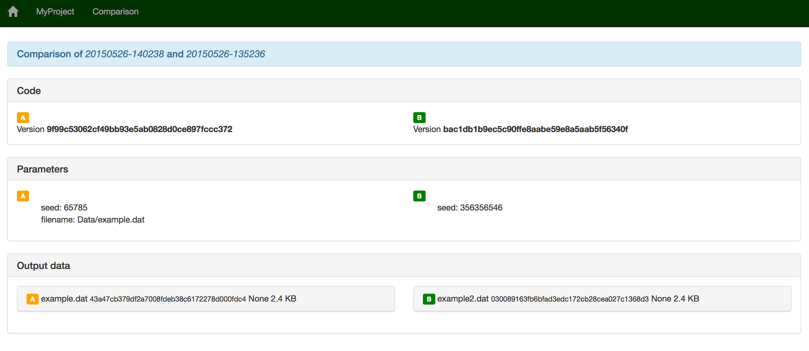
The web interface has also had a cosmetic update and several other improvements, including a more powerful comparison view (see screenshot). Importantly, the interface layout no longer breaks in narrower browser windows.

BSD licence

The Sumatra project aims to provide not only tools for scientists as end users (such as smt and smtweb), but also library components for developers to add Sumatra’s functionality to their own tools. To support this second use, we have switched licence from CeCILL (GPL-compatible) to the BSD 2-Clause Licence.

Python 3 support

In version 0.6.0, Sumatra already supported provenance capture for projects using Python 3, but required Python 2.6 or 2.7 to run. Thanks to Tim Tröndle, Sumatra now also runs in Python 3.4.

Plug-in interface

To support the wide diversity of workflows in scientific computing, Sumatra has always had an extensible architecture. It is intended to be easy to add support for new database formats, new programming languages, new version control systems, or new ways of launching computations.

Until now, adding such extensions has required that the code be included in Sumatra’s code base. Version 0.7.0 adds a plug-in interface, so you can define your own local extensions, or use other people’s.

For more information, see Extending Sumatra with plug-ins.

WebDAV support

The option to archive output data files has been extended to allow archiving to a remote server using the WebDAV protocol.

Support for the R language

Sumatra will now attempt to determine the versions of all external packages loaded by an R script.

Other changes

For developers, there has been a significant change - the project has moved from Mercurial to Git, and is now hosted on Github. Testing has also been significantly improved, with more system/integration testing, and the use of Docker for testing PostgreSQL and WebDAV support.

Parsing of command-line parameters has been improved. The ParameterSet classes now have a diff() method, making it easier to see the difference between two parameter sets, especially for large and hierarchical sets.

Following the recommendation of the Mercurial developers, and to enable the change of licence to BSD, we no longer use the Mercurial internal API. Instead we use the Mercurial command line interface via the hgapi package.

Bug fixes

A fair number of bugs have been fixed.

Download, support and documentation

The easiest way to get the latest version of Sumatra is

  $ pip install sumatra

Alternatively, Sumatra 0.7.0 may be downloaded from PyPI or from the INCF Software Center. Support is available from the sumatra-users Google Group. Full documentation is available on Read the Docs.

Elephant 0.1.0 released

We are pleased to announce the first release of the Elephant toolbox for the analysis of neurophysiology data.

Elephant builds on the Python scientific stack (NumPy, SciPy) to provide a set of well-tested analysis functions for spike train data and time series recordings from electrodes, such as spike train statistics, power spectrum analysis, filtering, cross-correlation and spike-triggered averaging. The toolbox also provides tools to generate artificial spike trains, either from stochastic processes or by controlled perturbations of real spike trains. Elephant is built on the Neo data model, and takes advantage of the broad file-format support provided by the Neo library. A bridge to the Pandas data analysis library is also provided.

Elephant is a community-based effort, aimed at providing a common platform to test and distribute code from different laboratories, with the goal of improving the reproducibility of modern neuroscience research. If you are a neuroscience researcher or student using Python for data analysis, please consider joining us, either to contribute your own code or to help with code review and testing.

Elephant is the direct successor to NeuroTools and maintains ties to complementary projects such as OpenElectrophy and SpykeViewer. It is also the default tool for electrophysiology data analysis in the Human Brain Project.

As a simple example, let's generate some artificial spike train data using a homogeneous Poisson process:

from elephant.spike_train_generation import homogeneous_poisson_process
from quantities import Hz, s, ms
spiketrains = [
    homogeneous_poisson_process(rate=10.0*Hz, t_start=0.0*s, t_stop=100.0*s)
    for i in range(100)]

and visualize it in Matplotlib:

import matplotlib.pyplot as plt
import numpy as np
for i, spiketrain in enumerate(spiketrains):
    t = spiketrain.rescale(ms)
    plt.plot(t, i * np.ones_like(t), 'k.', markersize=2)
plt.axis('tight')
plt.xlim(0, 1000)
plt.xlabel('Time (ms)', fontsize=16)
plt.ylabel('Spike Train Index', fontsize=16)
plt.gca().tick_params(axis='both', which='major', labelsize=14)
plt.show()
Now we calculate the coefficient of variation of the inter-spike interval for each of the 100 spike trains.

from elephant.statistics import isi, cv
cv_list = [cv(isi(spiketrain)) for spiketrain in spiketrains]

As expected for a Poisson process, the values cluster around 1:

plt.hist(cv_list)
plt.xlabel('CV', fontsize=16)
plt.ylabel('count', fontsize=16)
plt.gca().tick_params(axis='both', which='major', labelsize=14)
plt.show()

ANN: HoloViews 1.0 data visualization and ImaGen 2.0 pattern generation in Python

We are pleased to announce the first public release of HoloViews, a free Python package for scientific and engineering data visualization:

     http://ioam.github.io/holoviews

and version 2.0 of ImaGen, a free Python package for generating two-dimensional patterns useful for vision research and computational modeling:

     http://ioam.github.io/imagen

HoloViews provides composable, sliceable, declarative data structures for building even complex visualizations of any scientific data very easily.  With HoloViews, you can see your data as publication-quality figures almost instantly, so that you can focus on the data itself, rather than on laboriously putting together your figures.  Even complex multi-subfigure layouts and animations are very easily built using HoloViews.

ImaGen provides highly configurable, resolution-independent input patterns, directly visualizable using HoloViews but also available without any plotting package so that they can easily be incorporated directly into your computational modeling or visual stimulus generation code.  With ImaGen, any software with a Python interface can immediately support configurable streams of 0D, 1D, or 2D patterns, without any extra coding.

HoloViews and ImaGen are very general tools, but they were designed to solve common problems faced by vision scientists and computational modelers.  HoloViews makes it very easy to visualize data from vision research, whether it is visual patterns, neural activity patterns, or more abstract measurements or analyses.  Essentially, HoloViews provides a set of general, compositional, multidimensional data structures suitable for both discrete and continuous real-world data, and pairs them with separate customizable plotting classes to visualize them without extensive coding.

ImaGen 2.0 uses the continuous coordinate systems provided by HoloViews to implement flexible resolution-independent generation of streams of patterns, with parameters controlled by the user and allowing randomness or other arbitrary changes over time.  These patterns can be used for visual stimulus generation, testing or training computational models, initializing connectivity in models, or any other application where random or dynamic but precisely controlled streams of patterns are needed.

Features:

- Freely available under a BSD license
- Python 2 and 3 compatible
- Minimal external dependencies -- easy to integrate into your workflow
- Declarative approach provides powerful compositionality with minimal coding
- Include extensive, continuously tested IPython Notebook tutorials
- Easily reconfigurable using documented and validated parameters
- Animations are supported natively, with no extra work
- Supports reproducible research -- simple specification, archived in an IPython Notebook, providing a recipe for regenerating your results
- HoloViews is one of three winners of the 2015 UK Open Source Awards

To get started, check out ioam.github.io/holoviews and ioam.github.io/imagen!

Jean-Luc Stevens
Philipp Rudiger
Christopher Ball
James A. Bednar

Students: spend the summer improving brain research software tools in Google Summer of Code

From Malin Sandström at the INCF:

Are you a student interested in brain research and software development? Or do you know one?

This year again, INCF is participating as mentoring organization in the Google Summer of Code, a global program that offers students stipends to spend the summer writing code for open source projects. INCF has 27 project proposals offered by mentors from the international research community, many of them with a computational neuroscience slant. All projects deal with development and/or improvement of open source tools that are used in the neuroscience community.

You can see our full list of projects here: https://incf.org/gsoc/2015/proposals

To be eligible, students must fulfill the Google definition of 'student': an individual enrolled in or accepted into an accredited institution including (but not necessarily limited to) colleges, universities, masters programs, PhD programs and undergraduate programs.

Student applications open on Monday, March 16.

GSoC questions welcome to: gsoc@incf.org

Workshop Announcement - "HBP Hippocamp CA1: Collaborative and Integrative Modeling of Hippocampal Area CA1"

Registration is now open for the workshop "HBP Hippocamp CA1: Collaborative and Integrative Modeling of Hippocampal Area CA1", to be held March 31st - April 1st, 2015 at UCL School of Pharmacy in London, supported by the Human Brain Project (www.humanbrainproject.eu).

 In short, the aims of the workshop are two-fold. First, to engage the larger community of experimentalists and modelers working on hippocampus, and highlight existing modeling efforts and strategic datasets for modeling hippocampal area CA1. Second, to define and bootstrap an inclusive community-driven model and data-integration process to achieve open pre-competitive reference models of area CA1 (and, ultimately, the rest of the hippocampus), which are well documented, validated, and released at regular intervals (supported in part by IT infrastructure funded by HBP). Involvement from the community interested in characterization and modeling of the hippocampus is highly encouraged. To keep the meeting focused on the task, participation will be limited to ~30 people, so registration is required.

Please consult the meeting website at http://neuralensemble.org/meetings/HippocampCA1/ for registration and further details.

Organizing committee: Jo Falck (UCL), Szabolcs Káli (Hungarian Academy of Sciences), Sigrun Lange (UCL), Audrey Mercer (UCL), Eilif Muller (EPFL), Armando Romani (EPFL) and Alex Thomson (UCL).

PyNN 0.8 beta 2 released

We're happy to announce the second beta release of PyNN 0.8.

With this release we are getting close to a first release candidate: the NEST and NEURON backends are essentially feature complete, although with a few bugs remaining. If you're using one of these simulators as your PyNN backend we recommend using this beta release for new projects; now would also be a good time to think about upgrading existing projects. The Brian backend is less well developed, but considerable progress has been made.

For a list of the main changes between PyNN 0.7 and 0.8, see the release notes for the 0.8 alpha 1 release.

For the changes in this beta release see the release notes. In particular note that this release requires NEST version 2.4, and for the first time supports Python 3.2+ as well as Python 2.6 and 2.7. Support for NEST 2.6 will be provided in an upcoming release.

The source package is available from the INCF Software Center.

What is PyNN?

PyNN (pronounced 'pine' ) is a simulator-independent language for building neuronal network models.

In other words, you can write the code for a model once, using the PyNN API and the Python programming language, and then run it without modification on any simulator that PyNN supports (currently NEURON, NEST and Brian).

Even if you don't wish to run simulations on multiple simulators, you may benefit from writing your simulation code using PyNN's powerful, high-level interface. In this case, you can use any neuron or synapse model supported by your simulator, and are not restricted to the standard models.

PyNN is also being used as a user-friendly interface to neuromorphic hardware systems.

The code is released under the CeCILL licence (GPL-compatible).

GSoC Open Source Brain: Cortical Connections

Cortical Connections

In the same vein that the post before this one we will show here how to construct the connections between the cortical layers. In order to do so we will construct a function that works in general for any arbitrary connectivity, we describe in the following its structure. First, as in the thalamo-cortical connectivity, we have again the same structure of a function that loops over the target population extracting the relevant parameters that characterize these neurons. Furthermore we have another function that loops over the source population creating the corresponding tuples for the connection list. Is in this last function where the particular connectivity rule is implemented.

In the particular case of the Troyer model the connectivity between the cortical cells is determined by the correlation between the receptive fields of the neurons, the receptive fields here being Gabor functions. In more detail the neurons whose receptive fields are more correlated will be the ones more likely to have excitatory connections between them. On the other hand the ones whose receptive fields are less correlated will be more likely to receive inhibitory connections. In this post we show two schemes that accomplish this connectivity. The first one uses the fact the parameters of the receptive field to calculate a connectivity and the second one uses the receptive fields directly to calculate the correlations. We present the determining functions in the stated order down here.

Now we present the function that creates the connectivity for a given neuron par. The circular distance between the orientation and phases are calculated as a proxy to estimate how similar the receptive fields of the neurons are. After that, the distance between them is weighted and normalized with a normal function in order to obtain a value that we can interpret as a probability value. Finally in order to calculate the connectivity we sample n_pick times with the given probability value to see hwo strong a particular connection should be.

 
def cortical_to_cortical_connection(target_neuron_index, connections, source_population, n_pick, g, delay, source_orientations,
                                    source_phases, orientation_sigma, phase_sigma, target_neuron_orientation,
                                    target_neuron_phase, target_type):
    """
    Creates the connections from the source population to the target neuron

    """
    for source_neuron in source_population:
        # Extract index, orientation and phase of the target
        source_neuron_index = source_population.id_to_index(source_neuron)
        source_neuron_orientation = source_orientations[source_neuron_index]
        source_neuron_phase = source_phases[source_neuron_index]

        # Now calculate phase and orientation distances
        or_distance = circular_dist(target_neuron_orientation, source_neuron_orientation, 180)

        if target_type:
            phase_distance = circular_dist(target_neuron_phase, source_neuron_phase, 360)
        else:
            phase_distance = 180 - circular_dist(target_neuron_phase, source_neuron_phase, 360)

        # Now calculate the gaussian function
        or_gauss = normal_function(or_distance, mean=0, sigma=orientation_sigma)
        phase_gauss = normal_function(phase_distance, mean=0, sigma=phase_sigma)

        # Now normalize by guassian in zero
        or_gauss = or_gauss / normal_function(0, mean=0, sigma=orientation_sigma)
        phase_gauss = phase_gauss / normal_function(0, mean=0, sigma=phase_sigma)

        # Probability is the product
        probability = or_gauss * phase_gauss
        probability = np.sum(np.random.rand(n_pick) < probability)  # Samples
        synaptic_weight = (g / n_pick) * probability


        if synaptic_weight > 0:
                    connections.append((source_neuron_index, target_neuron_index, synaptic_weight, delay))

    return connections
      
    

Note that the overall strength is weighted by the conductivity value g that is passed as an argument. Furthermore a delay that is also passed as an argument is added to the list as the last element of the tuple.

Secondly we present the full correlation scheme. In this scheme we utilize the kernels directly to calculate the spatial correlation between them. In particular after we have flattened our kernels Z to have a series instead of a matrix we use the function perasonr from scipy.stats to calculate the correlation. Again as in the case above we use this probability to sample n_pick times and then calculate the relative connectivity strength with this.

 
def cortical_to_cortical_connection_corr(target_neuron_index, connections, source_population, n_pick, g, delay,
                                    source_orientations, source_phases, target_neuron_orientation, target_neuron_phase,
                                    Z1, lx, dx, ly, dy, sigma, gamma, w, target_type):
    """
    Creates the connections from the source population to the target neuron

    """
    for source_neuron in source_population:
        # Extract index, orientation and phase of the target
        x_source, y_source = source_neuron.position[0:2]
        source_neuron_index = source_population.id_to_index(source_neuron)
        source_neuron_orientation = source_orientations[source_neuron_index]
        source_neuron_phase = source_phases[source_neuron_index]

        Z2 = gabor_kernel(lx, dx, ly, dy, sigma, gamma, source_neuron_phase, w, source_neuron_orientation,
                          x_source, y_source)


        if target_type:
            probability = pearsonr(Z1.flat, Z2.flat)[0]
        else:
            probability = (-1) * pearsonr(Z1.flat, Z2.flat)[0]

        probability = np.sum(np.random.rand(n_pick) < probability)  # Samples
        synaptic_weight = (g / n_pick) * probability

        if synaptic_weight > 0:
                    connections.append((source_neuron_index, target_neuron_index, synaptic_weight, delay))

    return connections
    

Note that the overall strength is weighted by the conductivity value g that is passed as an argument. Furthermore a delay that is also passed as an argument is added to the list as the last element of the tuple.

We now show how a plot that illustrates how the probabilities change when the parameters that determined the gabor function are changed for each scheme.

In the figure above we have int he upper part how the probability for the first scheme a neuron with phase 0 and orientation 0 change as we vary the phase (left) and orientation (right). In the two graphs bellow we have the same for the second scheme we presented

GSoC Open Source Brain: Thalamo-Cortical Connections

Thalamo-cortical connections

In this post I will show how to build arbitrary custom connections in PyNN. We will illustrate the general technique in the particular case of the Troyer model. In the Troyer model the connections from the LGN to the cortex are determined with a gabor-profile therefore I am going to describe the required functions to achieve such an aim.

In the PyNN documentation we find that one of the ways of implementing arbitrary connectivity patterns is to use the FromListConnector utility. In this format we have to construct a list of tuples with a tuple for each connection. In each tuple we need to include the index of the source neuron (the neuron from which the synapse originates), the index of the target neuron (the neuron into which the synapse terminates), the weight and the delay. For example (0, 1, 5, 0.1) would indicate that we have a connection from the neuron 0 to the neuron 1 with a synaptic weight of 5 and a delay of 0.1.

In the light of the explanation above we need to construct a function that is able to construct a list with the appropriate weights given a target and a source populations. In order to start moving towards this goal we will first write a function that connects a given neuron in the target population to all the neurons in the source population. We first present the function here bellow and we will explain it later:

 
def lgn_to_cortical_connection(cortical_neuron_index, connections, lgn_neurons, n_pick, g, delay, polarity, sigma,
                               gamma, phi, w, theta, x_cortical, y_cortical):
    """
    Creates connections from the LGN to the cortex with a Gabor profile.

    This function adds all the connections from the LGN to the cortical cell with index = cortical_neuron_index. It
    requires as parameters the cortical_neruon_index, the current list of connections, the lgn population and also
    the parameters of the Gabor function.

    Parameters
    ----
    cortical_neuron_index : the neuron in the cortex -target- that we are going to connect to
    connections: the list with the connections to which we will append the new connnections
    lgn_neurons: the source population
    n_pick: How many times we will sample per neuron
    g: how strong is the connection per neuron
    delay: the time it takes for the action potential to arrive to the target neuron from the source neuron
    polarity: Whether we are connection from on cells or off cells
    sigma: Controls the decay of the exponential term
    gamma: x:y proportionality factor, elongates the pattern
    phi: Phase of the overall pattern
    w: Frequency of the pattern
    theta: Rotates the whole pattern by the angle theta
    x_cortical, y_cortical : The spatial coordinate of the cortical neuron

    """

    for lgn_neuron in lgn_neurons:
            # Extract position
            x, y = lgn_neuron.position[0:2]
            # Calculate the gabbor probability
            probability = polarity * gabor_probability(x, y, sigma, gamma, phi, w, theta, x_cortical, y_cortical)
            probability = np.sum(np.random.rand(n_pick) < probability)  # Samples

            synaptic_weight = (g / n_pick) * probability
            lgn_neuron_index = lgn_neurons.id_to_index(lgn_neuron)

            # The format of the connector list should be pre_neuron, post_neuron, w, tau_delay
            if synaptic_weight > 0:
                connections.append((lgn_neuron_index, cortical_neuron_index, synaptic_weight, delay))

    

The first thing to note from the function above are its arguments. It contains the source population and the particular target neuron that we want to connect to. It also contains all the connectivity and gabor-function related parameters. In the body of the function we have one loop over the whole source population that decides whether we add a connection from a particular cell or not. In order to decide if we add a connection we have to determine the probability from the gabor function. Once we have this we sample n_pick times and add a weighted synaptic weight accordingly to the list for each neuron.

In the function above we have the values of the gabor function passed as arguments. However, the values of each gabor function depend on the nature of the cell of the target population. In the light of this we will construct another function that loops over the target population and extracts the appropriate gabor values for each function in this population. We again present the function and then explain it:

def create_lgn_to_cortical(lgn_population, cortical_population, polarity,  n_pick, g, delay,  sigma, gamma, phases,
                           w, orientations):
    """
    Creates the connection from the lgn population to the cortical population with a gabor profile. It also extracts
    the corresponding gabor parameters that are needed in order to determine the connectivity.
    """

    print 'Creating connection from ' + lgn_population.label + ' to ' + cortical_population.label

    # Initialize connections
    connections = []

    for cortical_neuron in cortical_population:
        # Set the parameters
        x_cortical, y_cortical = cortical_neuron.position[0:2]
        cortical_neuron_index = cortical_population.id_to_index(cortical_neuron)
        theta = orientations[cortical_neuron_index]
        phi = phases[cortical_neuron_index]

        # Create the connections from lgn to cortical_neuron
        #lgn_to_cortical_connection(cortical_neuron_index, connections, lgn_population, n_pick, g, polarity, sigma,
        #gamma, phi, w, theta, x_cortical, y_cortical)

        lgn_to_cortical_connection(cortical_neuron_index, connections, lgn_population, n_pick, g, delay, polarity, sigma,
                                   gamma, phi, w, theta, 0, 0)

    return connections
    

This function requires as arguments the source and target populations as well as the necessary parameters that characterize each cell connectivity: orientation and phase. In the body of the function we have a loop over the cortical population that extracts the relevant parameters -position, orientation and phase- and then calls the function that we already describe previously in order to create the connectivity from the source population to the cell in place.

So now we have the necessary functions to construct a list. Now, we can use FromListConnector to transform the list into a connector. And the use this to define a Projection. We define both the excitatory and inhibitory connections. We abstract this complete set into the following function:

def create_thalamocortical_connection(source, target, polarity, n_pick, g, delay, sigma, gamma, w, phases, orientations, simulator):
    """
    Creates a connection from a layer in the thalamus to a layer in the cortex through the mechanism of Gabor sampling
    """

    # Produce a list with the connections
    connections_list = create_lgn_to_cortical(source, target, polarity, n_pick, g, delay, sigma, gamma, phases, w, orientations)

    # Transform it into a connector
    connector = simulator.FromListConnector(connections_list, column_names=["weight", "delay"])

    # Create the excitatory and inhibitory projections
    simulator.Projection(source, target, connector, receptor_type='excitatory')
    simulator.Projection(source, target, connector, receptor_type='inhibitory')      
    

With this we can create in general connections from one target population to the other. We can even change change the gabor function for whatever we want if we want to experiment with other connectivity patterns. Finally we present down here an example of a sampling from a Gabor function with the aglorithm we just constructed:

So in the image we show in the left the sampling from the ideal Gabor function in the right.